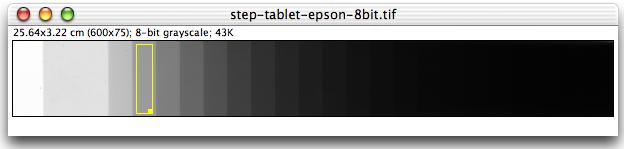
Figure 1. Optical density step tablet.
Figure 1 is a Kodak No. 3 Calibrated Step Tablet scanned with an Epson Expression 1680 Professional scanner. The tablet has 21 steps with a density range of 0.05 to 3.05 OD. This image is available as a ZIP compressed TIFF file that can be opened directly in ImageJ. Calibrated step tablets are available from Tiffen (Kodak) and Stouffer.
The first step in calibrating the image is to measure the mean gray value of the background and the first 18 steps. We don't measure the last three steps be because they are not distinguishable and also because the calibration function in ImageJ is currently limited to 20 measurements. Before starting, make sure the "Results" window is closed. Create a rectangular selection that fills most of one step without overlapping another step. Move the selection to the white background at the left end of the image and measure it. Then, starting at the left, move the selection and measure each of the first 18 steps.
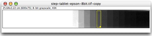
Figure 2. OD step tablet with adjusted LUT.
About half way through the process of measuring the steps, use the Image/Adjust/Brightness/Contrast tool to adjust the LUT so that the darker steps on the right side of the tablet are visible. There should be 19 measurements listed in the "Results" window when you are finished.
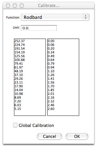
Figure 3. Analyze/Calibrate dialog box.
Open the Analyze/Calibrate dialog box and you will see that the 19 measurements have been automatically entered into the left column. Paste the following OD values into the right column, select "Rodbard" from the "Function" popup menu, enter "O.D." into the "Unit" field, then press "OK". ImageJ will then generate and display the calibration curve.
0.00
0.06
0.20
0.34
0.49
0.64
0.79
0.94
1.10
1.26
1.41
1.56
1.70
1.85
2.01
2.16
2.32
2.46
2.60
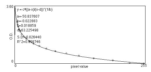
Figure 4. Calibration curve.
The image is now calibrated to optical density. Save the image in TIFF format and the calibration curve will be saved with it. You can use the same calibration curve with all open images by checking "Global Calibration" in the Analyze/Calibrate dialog box.
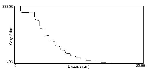
Figure 5. Profile plot of uncalibrated image.
Before calibration, pixel values are in gray level units in the range 0-255. After calibration, pixel values are in OD.
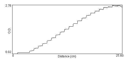
Figure 6. Profile plot of calibrated image.